 SciGalaxy Tutorial
Views
What each layout shows, and a sentence you can adapt for a paper.
One run can be read in several layouts. The top bar is the cluster map, timeline, timezone, circle, landscape, heatmap, and t-SNE. Cluster evolution, structural variation, and entropy are under Cluster evolution. Geography and the dual-map overlay are under Overlay and map.
Each section says what to look at, then gives a sentence you can adapt. Replace the blank with a number from your run. You do not have to draft the methods paragraph by hand. The export page writes it from the settings. See Export and writing.
Cluster map
Look for the groups: which nodes connect, where the large nodes sit, and which group holds the red rings. This is the force-directed layout, and it is the default.
In a paper: Louvain clustering produced the thematic groups. Modularity Q was ……, and the mean silhouette S was ……. The silhouette is still being calibrated against CiteSpace, so name SciGalaxy as the tool that produced S.
The symbols on this view are in How to read the map.
Timeline
Each row is a cluster, and the axis runs from early years to late ones. Use it to see when a theme acquires its landmark references, whether there is a gap, and whether the bursts fall early or late.
In a paper: The timeline places one cluster on each row. The highly cited nodes of a given theme concentrate around ……, and the bursts fall between …… and …….
Timezone
Each column is the year a node first enters the network. Use it for the year a term arrives, not for how long it keeps being cited afterwards.
In a paper: The timezone view columns nodes by the year they first appear. Labels for one theme arrive late in the window, which marks a late entry into the literature.
Circle
Each cluster takes an arc of a ring, and its nodes sit on that arc. Groups that pile up in the force layout separate here. The clustering is unchanged. Only the layout changes.
In a paper: The same clusters are shown on a circle, one arc per cluster, so that groups which overlap in the force-directed layout can be read separately.
Landscape
Density is drawn as terrain. A peak is a crowd of nodes. A valley is a sparse patch. The ramp runs from low density to high density. If the graph has no saved layout, the coordinates are computed with a force layout.
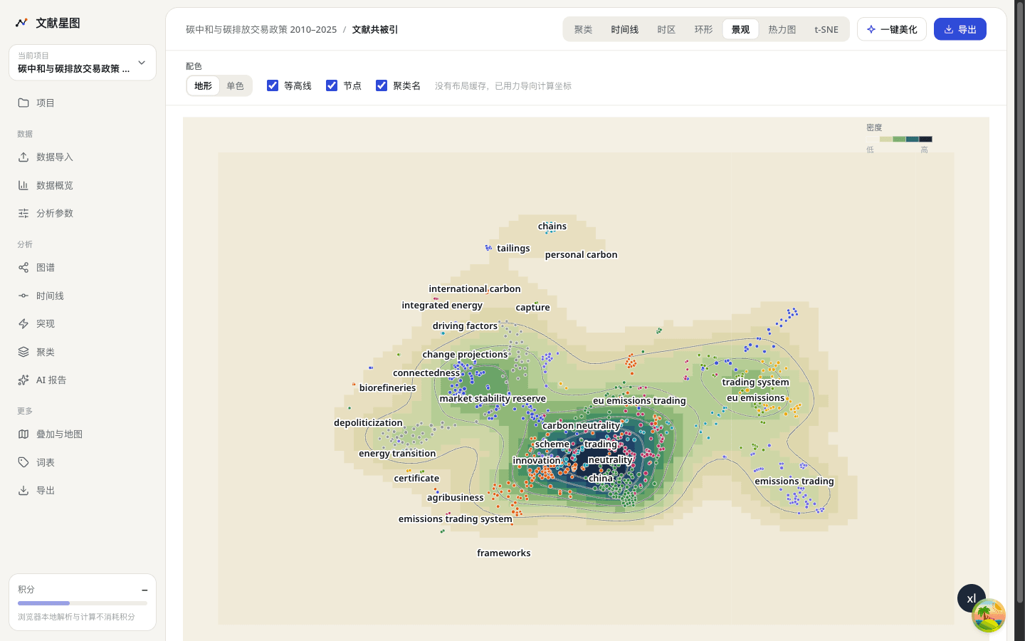
In a paper: The landscape draws network density as a contour surface. The highest peak corresponds to …….
Heatmap
Rows are clusters or nodes. Columns are years. Color is frequency. Absolute values show the raw count. Row normalization shows where that row peaks, regardless of how large the row is. When there are many nodes, the heatmap keeps the ones at the top of the current sort.
In a paper: The heatmap crosses clusters (or nodes) with years. Frequency for one theme peaks in …….
t-SNE
Nodes are projected onto a plane from the links in the network. Tightly linked nodes land near each other. The projection does not recompute the clusters. On a large network, the highest-frequency nodes are kept and the rest are left out of the projection.
In a paper: A t-SNE projection shows which nodes sit near each other. Proximity reflects link structure. Cluster membership remains the Louvain partition.
Cluster evolution
The alluvial diagram cuts the time span into periods, clusters each period, and draws ribbons between them. A ribbon that continues is a theme that carries on. A ribbon that splits is a theme breaking apart. Ribbons that join are a merge. Each period is labeled with its own Q.
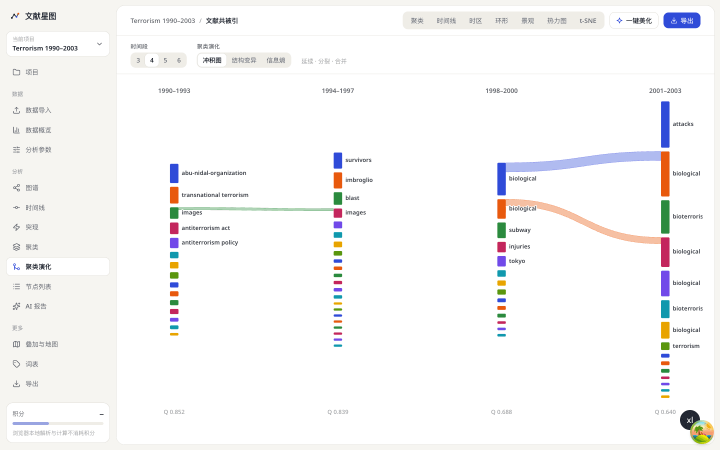
In a paper: Cluster evolution is shown as an alluvial diagram. One theme continues until …… and then splits into …… and …….
Structural variation
Structural variation (SVA) scores citing papers, not the nodes. It looks for papers whose references change the network that was already there: for example by linking clusters that did not previously touch, or by shifting modularity. Run it after an intellectual-base or document co-citation analysis when you want the papers that may be rearranging the field.
In a paper: Structural variation analysis flagged citing papers that altered the existing co-citation structure. The highest-ranked papers link themes that had been separate.
Entropy
Entropy measures how spread out the frequencies are inside each time slice. A rise means attention is scattering across more nodes. A fall means it is concentrating. A flat line means the concentration did not change much.
In a paper: Information entropy across the slices rises (or falls), which indicates that themes in this span are scattering (or concentrating).
Geography
The map places countries and regions from the addresses in the records. Arcs are collaborations between countries. Darker marks mean more papers. A ranked list sits under the map. Institutions are plotted when a coordinate can be resolved. Addresses that cannot be recognized stay on an unresolved list. They are not assigned to a country.
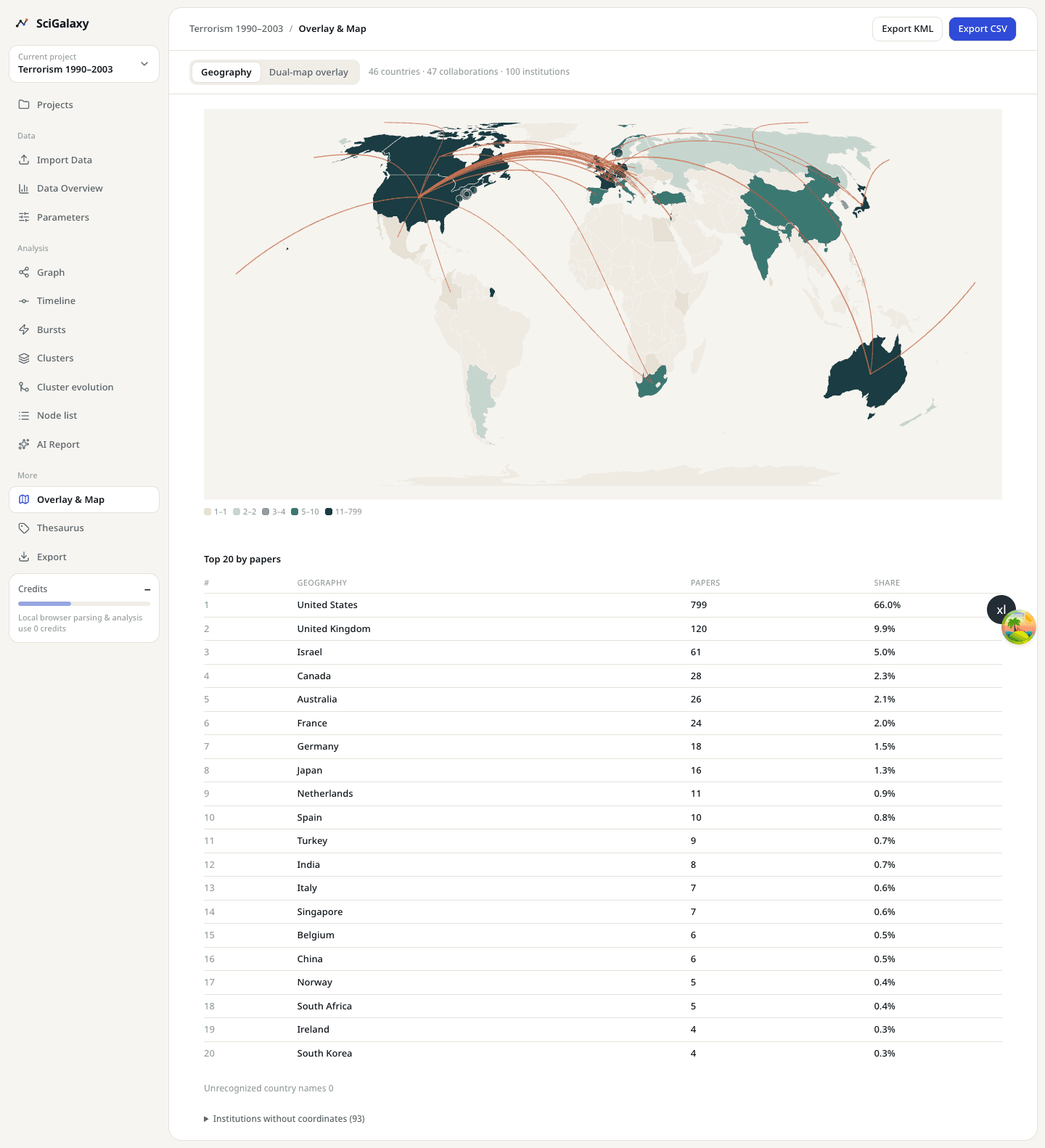
In a paper: The geographic map shows publication counts and international collaboration. The largest contributions come from ……, and the collaboration arcs run mainly between …… and …….
Dual-map overlay
Both panels use one basemap, built from the OpenAlex subject system. It is not the CiteSpace JCR basemap. One side is the subject of the citing papers. The other side is the subject of the cited work. Point size is a paper count or a citation count. Arcs are the stronger citation paths, and they show which subjects the citations leave and which subjects they land in.
In a paper: The dual-map overlay uses the OpenAlex subject system. Citing papers fall mainly in ……, while their references come from ……, with a stronger citation path between the two.
Figure formats for these views are in Export and writing.